Exploratory analysis on suicide data
Suicide analysis
import numpy as np
import pandas as pd
import matplotlib.pyplot as plt
import seaborn as sns

%matplotlib inline
Reading the data
df = pd.read_csv('master.csv')
Let’s take a look at the data:
df.sample(5)
| country | year | sex | age | suicides_no | population | suicides/100k pop | country-year | HDI for year | gdp_for_year ($) | gdp_per_capita ($) | generation | |
|---|---|---|---|---|---|---|---|---|---|---|---|---|
| 12171 | Ireland | 1994 | female | 15-24 years | 13 | 303000 | 4.29 | Ireland1994 | NaN | 57,166,037,102 | 17188 | Generation X |
| 11049 | Guatemala | 2014 | female | 5-14 years | 13 | 1906536 | 0.68 | Guatemala2014 | 0.627 | 58,722,323,918 | 4210 | Generation Z |
| 23290 | South Africa | 1996 | male | 35-54 years | 36 | 4031071 | 0.89 | South Africa1996 | NaN | 147,607,982,695 | 3908 | Boomers |
| 7902 | Ecuador | 2002 | male | 55-74 years | 39 | 525419 | 7.42 | Ecuador2002 | NaN | 28,548,945,000 | 2472 | Silent |
| 5936 | Colombia | 2010 | male | 75+ years | 65 | 418296 | 15.54 | Colombia2010 | 0.706 | 287,018,184,638 | 6836 | Silent |
df.describe()
| year | suicides_no | population | suicides/100k pop | HDI for year | gdp_per_capita ($) | |
|---|---|---|---|---|---|---|
| count | 27820.000000 | 27820.000000 | 2.782000e+04 | 27820.000000 | 8364.000000 | 27820.000000 |
| mean | 2001.258375 | 242.574407 | 1.844794e+06 | 12.816097 | 0.776601 | 16866.464414 |
| std | 8.469055 | 902.047917 | 3.911779e+06 | 18.961511 | 0.093367 | 18887.576472 |
| min | 1985.000000 | 0.000000 | 2.780000e+02 | 0.000000 | 0.483000 | 251.000000 |
| 25% | 1995.000000 | 3.000000 | 9.749850e+04 | 0.920000 | 0.713000 | 3447.000000 |
| 50% | 2002.000000 | 25.000000 | 4.301500e+05 | 5.990000 | 0.779000 | 9372.000000 |
| 75% | 2008.000000 | 131.000000 | 1.486143e+06 | 16.620000 | 0.855000 | 24874.000000 |
| max | 2016.000000 | 22338.000000 | 4.380521e+07 | 224.970000 | 0.944000 | 126352.000000 |
The dataset has data from suicides from 1985 to 2016.
df.info()
<class 'pandas.core.frame.DataFrame'>
RangeIndex: 27820 entries, 0 to 27819
Data columns (total 12 columns):
country               27820 non-null object
year                  27820 non-null int64
sex                   27820 non-null object
age                   27820 non-null object
suicides_no           27820 non-null int64
population            27820 non-null int64
suicides/100k pop     27820 non-null float64
country-year          27820 non-null object
HDI for year          8364 non-null float64
 gdp_for_year ($)     27820 non-null object
gdp_per_capita ($)    27820 non-null int64
generation            27820 non-null object
dtypes: float64(2), int64(4), object(6)
memory usage: 2.5+ MB
is there null data?
df.isnull().sum()
country                   0
year                      0
sex                       0
age                       0
suicides_no               0
population                0
suicides/100k pop         0
country-year              0
HDI for year          19456
 gdp_for_year ($)         0
gdp_per_capita ($)        0
generation                0
dtype: int64
Understanding the data
The country-year field displays the country name and year of the record. In this way, it is a redundant field and will be discarded. Also due to most data from the ‘HDI for year’ field, it will be discarded.
df.drop(['country-year', 'HDI for year'], inplace=True, axis = 1)
Let’s rename some columns simply to make it easier to access them.
df = df.rename(columns={'gdp_per_capita ($)': 'gdp_per_capita', ' gdp_for_year ($) ':'gdp_for_year'})
In this case, the ‘gdp_for_year’ field is as a string, so let’s convert this to a number.
for i, x in enumerate(df['gdp_for_year']):
    df['gdp_for_year'][i] = x.replace(',', '')

df['gdp_for_year'] = df['gdp_for_year'].astype('int64')
Data Description
Each data in the data set represents a year, a country, a certain age range, and a gender. For example, in the country Brazil in the year 1985, over 75 years, committed suicide 129 men.
The data set has 10 attributes. These being:
- Country: country of record data;
- Year: year of record data;
- Sex: Sex (male or female);
- Age: Suicide age range, ages divided into six categories;
- Suicides_no: number of suicides;
- Population: population of this sex, in this age range, in this country and in this year;
- Suicides / 100k pop: Reason between the number of suicides and the population / 100k;
- GDP_for_year: GDP of the country in the year who issue;
- GDP_per_capita: ratio between the country’s GDP and its population;
- Generation: Generation of the suicides in question, being possible 6 different categories.
Possible age categories and generations are:
df['age'].unique()
array(['15-24 years', '35-54 years', '75+ years', '25-34 years',
       '55-74 years', '5-14 years'], dtype=object)
df['generation'].unique()
array(['Generation X', 'Silent', 'G.I. Generation', 'Boomers',
       'Millenials', 'Generation Z'], dtype=object)
Adding some things
As the HDI was discarded and it is very interesting to assess whether the development of the country has an influence on the suicide rate, I have separated a list of first and second world countries from the data of the site:
http://worldpopulationreview.com
Then I categorized each country in the data set into first, second and third world.
Frist_world = ['United States', 'Germany', 'Japan', 'Turkey', 'United Kingdom', 'France', 'Italy', 'South Korea',
              'Spain', 'Canada', 'Australia', 'Netherlands', 'Belgium', 'Greece', 'Portugal',
              'Sweden', 'Austria', 'Switzerland', 'Israel', 'Singapore', 'Denmark', 'Finland', 'Norway', 'Ireland',
              'New Zeland', 'Slovenia', 'Estonia', 'Cyprus', 'Luxembourg', 'Iceland']

Second_world = ['Russian Federation', 'Ukraine', 'Poland', 'Uzbekistan', 'Romania', 'Kazakhstan', 'Azerbaijan', 'Czech Republic',
               'Hungary', 'Belarus', 'Tajikistan', 'Serbia', 'Bulgaria', 'Slovakia', 'Croatia', 'Maldova', 'Georgia',
               'Bosnia And Herzegovina', 'Albania', 'Armenia', 'Lithuania', 'Latvia', 'Brazil', 'Chile', 'Argentina',
               'China', 'India', 'Bolivia', 'Romenia']
country_world = []
for i in range(len(df)):

    if df['country'][i] in Frist_world:
        country_world.append('1')
    elif df['country'][i] in Second_world:
        country_world.append('2')
    else:
        country_world.append('3')

df['country_world'] = country_world
Exploratory analysis
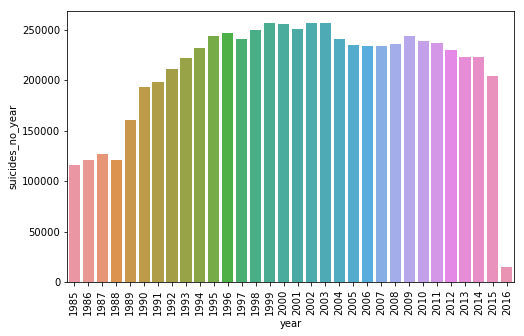
I will analyze the impact of some attributes on the amount of suicides. We start this year.
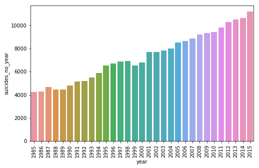
Year
suicides_no_year = []

for y in df['year'].unique():
    suicides_no_year.append(sum(df[df['year'] == y]['suicides_no']))

n_suicides_year = pd.DataFrame(suicides_no_year, columns=['suicides_no_year'])
n_suicides_year['year'] = df['year'].unique()

top_year = n_suicides_year.sort_values('suicides_no_year', ascending=False)['year']
top_suicides = n_suicides_year.sort_values('suicides_no_year', ascending=False)['suicides_no_year']

plt.figure(figsize=(8,5))
plt.xticks(rotation=90)
sns.barplot(x = top_year, y = top_suicides)
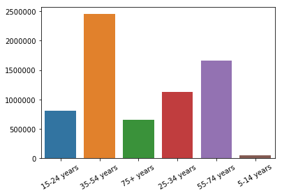
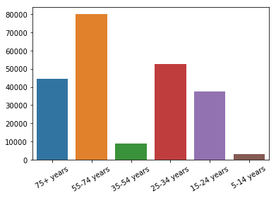
Age
suicides_no_age = []

for a in df['age'].unique():
    suicides_no_age.append(sum(df[df['age'] == a]['suicides_no']))

plt.xticks(rotation=30)
sns.barplot(x = df['age'].unique(), y = suicides_no_age)
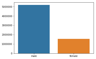
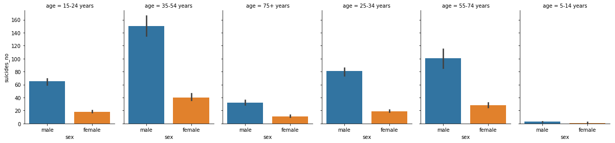
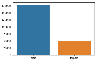
Sex
suicides_no_sex = []

for s in df['sex'].unique():
    suicides_no_sex.append(sum(df[df['sex'] == s]['suicides_no']))

sns.barplot(x = df['sex'].unique(), y = suicides_no_sex)
<matplotlib.axes._subplots.AxesSubplot at 0x7ff84a0f1b00>
sns.catplot(x='sex', y='suicides_no',col='age', data=df, estimator=np.median,height=4, aspect=.7,kind='bar')
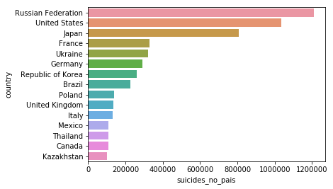
Country
Countries with larger populations should have more suicides.
suicides_no_pais = []
for c in df['country'].unique():
    suicides_no_pais.append(sum(df[df['country'] == c]['suicides_no']))

n_suicides_pais = pd.DataFrame(suicides_no_pais, columns=['suicides_no_pais'])
n_suicides_pais['country'] = df['country'].unique()

quant = 15
top_paises = n_suicides_pais.sort_values('suicides_no_pais', ascending=False)['country'][:quant]
top_suicides = n_suicides_pais.sort_values('suicides_no_pais', ascending=False)['suicides_no_pais'][:quant]
sns.barplot(x = top_suicides, y = top_paises)
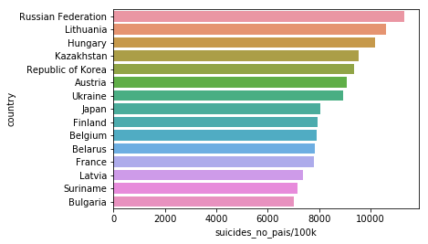
By using the amount of suicides per 100k inhabitants, we remove the bias of overpopulated countries.
suicides_no_pais = []
for c in df['country'].unique():
    suicides_no_pais.append(sum(df[df['country'] == c]['suicides/100k pop']))

n_suicides_pais = pd.DataFrame(suicides_no_pais, columns=['suicides_no_pais/100k'])
n_suicides_pais['country'] = df['country'].unique()

quant = 15
top_paises = n_suicides_pais.sort_values('suicides_no_pais/100k', ascending=False)['country'][:quant]
top_suicides = n_suicides_pais.sort_values('suicides_no_pais/100k', ascending=False)['suicides_no_pais/100k'][:quant]
sns.barplot(x = top_suicides, y = top_paises)
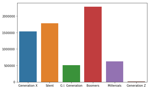
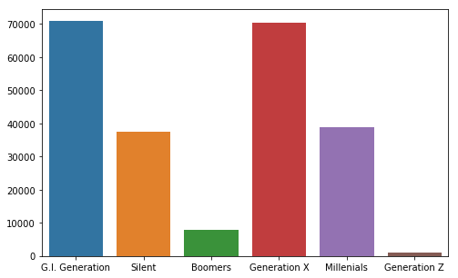
Generation
suicides_no_gen = []
for g in df['generation'].unique():
    suicides_no_gen.append(sum(df[df['generation'] == g]['suicides_no']))

plt.figure(figsize=(8,5))
sns.barplot(x = df['generation'].unique(), y = suicides_no_gen)
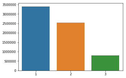
Country world
suicides_no_world = []
for w in df['country_world'].unique():
    suicides_no_world.append(sum(df[df['country_world'] == w]['suicides_no']))

sns.barplot(x = df['country_world'].unique(), y = suicides_no_world)
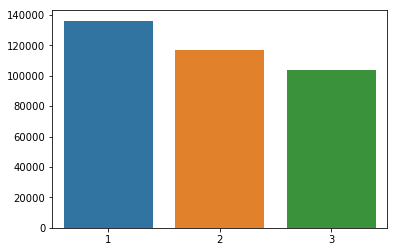
suicides_no_world = []
for w in df['country_world'].unique():
    suicides_no_world.append(sum(df[df['country_world'] == w]['suicides/100k pop']))

sns.barplot(x = df['country_world'].unique(), y = suicides_no_world)
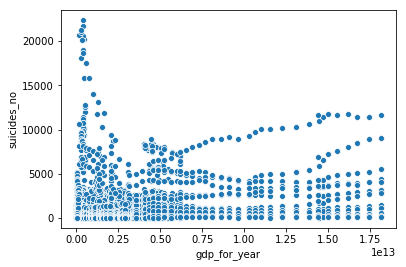
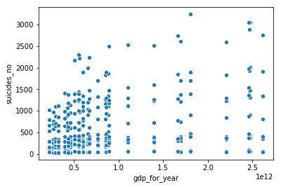
GDP for year
sns.scatterplot(x = 'gdp_for_year', y = 'suicides_no', data = df)
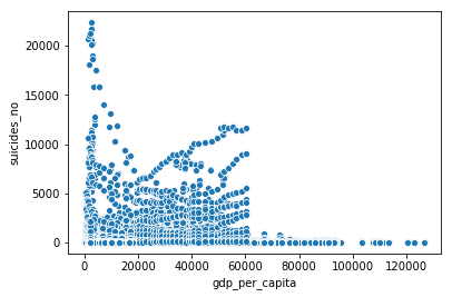
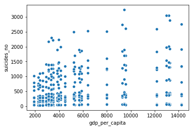
GDP por capita
sns.scatterplot(x = 'gdp_per_capita', y = 'suicides_no', data = df)
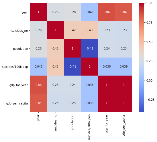
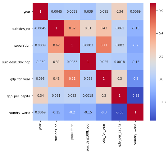
Attribute Correlation
plt.figure(figsize=(8,7))
sns.heatmap(df.corr(), cmap = 'coolwarm', annot=True)
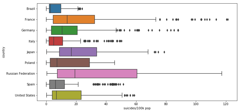
Checking the suicidade/100k distribution of some countries
countries = ['Russian Federation', 'Brazil', 'Poland', 'Italy', 'United States', 'Germany', 'Japan', 'Spain', 'France']
df_filtred = df[[df['country'][i] in countries for i in range(len(df))]]

plt.figure(figsize=(12,6))
sns.boxplot(x = 'suicides/100k pop', y = 'country', data = df_filtred)
General Plot of the World
import plotly.plotly as py
import plotly.graph_objs as go
from plotly.offline import download_plotlyjs, init_notebook_mode, plot, iplot
init_notebook_mode(connected=True)
cod = pd.read_csv('https://raw.githubusercontent.com/plotly/datasets/master/2014_world_gdp_with_codes.csv')
codes = []
for i in range(len(n_suicides_pais)):
    c = n_suicides_pais['country'][i]
    f = 0
    for j in range(len(cod)):
        if c == cod['COUNTRY'][j]:
            tmp = cod['CODE'][j]
            f = 1
            break
    if f == 0:
        if c == 'Bahamas':
            tmp  = 'BHM'
        elif c == 'Republic of Korea':
            tmp = 'KOR'
        elif c == 'Russian Federation':
            tmp = 'RUS'
        else:
            tmp = 'VC'
    codes.append(tmp)
data = dict(
        type = 'choropleth',
        locations = codes,
        z = n_suicides_pais['suicides_no_pais/100k'],
        text = n_suicides_pais['country'],
        colorbar = {'title' : 'número de suicídios'},
      )
layout = dict(
    title = 'Mapa de calor de suicídios 1985-2016',
    geo = dict(
        showframe = False,
        projection = {'type':'equirectangular'}
    )
)
choromap = go.Figure(data = [data],layout = layout)
iplot(choromap)
Brazil Facts
As a Brazilian, I have a particular interest in the suicide rate in Brazil. So I’m going to try to analyze the specific indices of this country.
df_brasil = df[df['country'] == 'Brazil']
Country and country fields are all the same, then discarded.
df_brasil.drop(['country', 'country_world'], axis = 1, inplace = True)
I’m going to repeat a lot of the graphics already done.
suicides_no_year = []

for y in df_brasil['year'].unique():
    suicides_no_year.append(sum(df_brasil[df_brasil['year'] == y]['suicides_no']))

n_suicides_year = pd.DataFrame(suicides_no_year, columns=['suicides_no_year'])
n_suicides_year['year'] = df_brasil['year'].unique()

top_year = n_suicides_year.sort_values('suicides_no_year', ascending=False)['year']
top_suicides = n_suicides_year.sort_values('suicides_no_year', ascending=False)['suicides_no_year']

plt.figure(figsize=(8,5))
plt.xticks(rotation=90)
sns.barplot(x = top_year, y = top_suicides)
suicides_no_age = []

for a in df['age'].unique():
    suicides_no_age.append(sum(df_brasil[df_brasil['age'] == a]['suicides_no']))

plt.xticks(rotation=30)
sns.barplot(x = df_brasil['age'].unique(), y = suicides_no_age)
suicides_no_sex = []

for s in df['sex'].unique():
    suicides_no_sex.append(sum(df_brasil[df_brasil['sex'] == s]['suicides_no']))

sns.barplot(x = df_brasil['sex'].unique(), y = suicides_no_sex)
suicides_no_gen = []
for g in df['generation'].unique():
    suicides_no_gen.append(sum(df_brasil[df_brasil['generation'] == g]['suicides_no']))

plt.figure(figsize=(8,5))
sns.barplot(x = df_brasil['generation'].unique(), y = suicides_no_gen)
sns.scatterplot(x = 'gdp_for_year', y = 'suicides_no', data = df_brasil)
sns.scatterplot(x = 'gdp_per_capita', y = 'suicides_no', data = df_brasil)
plt.figure(figsize=(8,7))
sns.heatmap(df_brasil.corr(), cmap = 'coolwarm', annot=True)