
Fraud detection - Unsupervised Anomaly Detection
Fraud detection - Unsupervised Anomaly Detection
An 100% unsupervised approach to discover frauds on credit card transactions

One of the greatest concerns of many business owners is how to protect their company from fraudulent activity. This concern motivated large companies to save data relative to their past frauds, however whomever performs a fraud aims not to be caught then this kind of data usualy is unlabeled or partially labeled.
On this article, we will talk about how to discover frauds on a credit card transaction dataset, unlike most fraud datasets this dataset is completely labeled however, we won’t use the label to discover frauds. Credit card fraud is when someone uses another person’s credit card or account information to make unauthorized purchases or access funds through cash advances. Credit card fraud doesn’t just happen online; it happens in brick-and-mortar stores, too. As a business owner, you can avoid serious headaches - and unwanted publicity - by recognizing potentially fraudulent use of credit cards in your payment environment.
One of the most common approach to find fraudulent transactions was randomly select some transactions and ask and auditor to audit it. This approach was quite unaccurate since the relation between the number of fraudulent transactions and normal transactions is close to 0.1%.
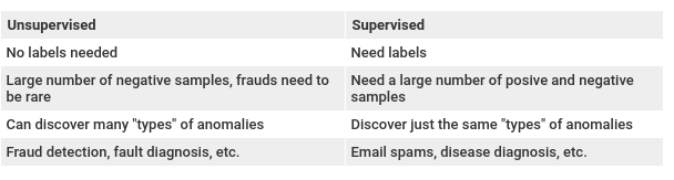
Then, we aim to leverage machine learning to detect and prevent frauds and make fraud fighters more efficient and effective. Comumly, there are the supervised and the unsupervised approach:
Also, these models can then be deployed to automatically identify new instances/cases of known fraud patterns/types in the future. Ideally the validation of this type of machine learning algorith sometimes need to be a temporal validation since fraud patterns can change over time, however to simplify this article, the validation will be simplified.
import pandas as pd
import numpy as np
import matplotlib.pyplot as plt
import seaborn as sns
from sklearn.manifold import TSNE
from sklearn.decomposition import PCA
from sklearn.model_selection import train_test_split
from sklearn.metrics import mean_squared_error, classification_report
from sklearn.preprocessing import StandardScaler
from tensorflow.keras.layers import Input, Dense
from tensorflow.keras.models import Model, Sequential
from tensorflow.keras.optimizers import Adam

%matplotlib inline
Data description
The project uses a dataset of around 284000 credit card transactions which have been taken from Kaggle.
The dataset is highly unbalanced, the positive class (frauds) account for 0.172% of all transactions. It contains only numerical input variables which are the result of a PCA transformation. Unfortunately, due to confidentiality issues, the original features and more background information about the data are not provided. Features V1, V2, …, V28 are the principal components obtained with PCA, the only features which have not been transformed with PCA are “Time” and “Amount”, and there are no null values (Dataset page).
df = pd.read_csv("creditcard.csv")
df.shape
(284807, 31)
df["Time"] = df["Time"].apply(lambda x : x / 3600 % 24)
df.describe().T
| count | mean | std | min | 25% | 50% | 75% | max | |
|---|---|---|---|---|---|---|---|---|
| Time | 284807.0 | 1.453795e+01 | 5.847061 | 0.000000 | 10.598194 | 15.010833 | 19.329722 | 23.999444 |
| V1 | 284807.0 | 1.165980e-15 | 1.958696 | -56.407510 | -0.920373 | 0.018109 | 1.315642 | 2.454930 |
| V2 | 284807.0 | 3.416908e-16 | 1.651309 | -72.715728 | -0.598550 | 0.065486 | 0.803724 | 22.057729 |
| V3 | 284807.0 | -1.373150e-15 | 1.516255 | -48.325589 | -0.890365 | 0.179846 | 1.027196 | 9.382558 |
| V4 | 284807.0 | 2.086869e-15 | 1.415869 | -5.683171 | -0.848640 | -0.019847 | 0.743341 | 16.875344 |
| V5 | 284807.0 | 9.604066e-16 | 1.380247 | -113.743307 | -0.691597 | -0.054336 | 0.611926 | 34.801666 |
| V6 | 284807.0 | 1.490107e-15 | 1.332271 | -26.160506 | -0.768296 | -0.274187 | 0.398565 | 73.301626 |
| V7 | 284807.0 | -5.556467e-16 | 1.237094 | -43.557242 | -0.554076 | 0.040103 | 0.570436 | 120.589494 |
| V8 | 284807.0 | 1.177556e-16 | 1.194353 | -73.216718 | -0.208630 | 0.022358 | 0.327346 | 20.007208 |
| V9 | 284807.0 | -2.406455e-15 | 1.098632 | -13.434066 | -0.643098 | -0.051429 | 0.597139 | 15.594995 |
| V10 | 284807.0 | 2.239751e-15 | 1.088850 | -24.588262 | -0.535426 | -0.092917 | 0.453923 | 23.745136 |
| V11 | 284807.0 | 1.673327e-15 | 1.020713 | -4.797473 | -0.762494 | -0.032757 | 0.739593 | 12.018913 |
| V12 | 284807.0 | -1.254995e-15 | 0.999201 | -18.683715 | -0.405571 | 0.140033 | 0.618238 | 7.848392 |
| V13 | 284807.0 | 8.176030e-16 | 0.995274 | -5.791881 | -0.648539 | -0.013568 | 0.662505 | 7.126883 |
| V14 | 284807.0 | 1.206296e-15 | 0.958596 | -19.214325 | -0.425574 | 0.050601 | 0.493150 | 10.526766 |
| V15 | 284807.0 | 4.913003e-15 | 0.915316 | -4.498945 | -0.582884 | 0.048072 | 0.648821 | 8.877742 |
| V16 | 284807.0 | 1.437666e-15 | 0.876253 | -14.129855 | -0.468037 | 0.066413 | 0.523296 | 17.315112 |
| V17 | 284807.0 | -3.800113e-16 | 0.849337 | -25.162799 | -0.483748 | -0.065676 | 0.399675 | 9.253526 |
| V18 | 284807.0 | 9.572133e-16 | 0.838176 | -9.498746 | -0.498850 | -0.003636 | 0.500807 | 5.041069 |
| V19 | 284807.0 | 1.039817e-15 | 0.814041 | -7.213527 | -0.456299 | 0.003735 | 0.458949 | 5.591971 |
| V20 | 284807.0 | 6.406703e-16 | 0.770925 | -54.497720 | -0.211721 | -0.062481 | 0.133041 | 39.420904 |
| V21 | 284807.0 | 1.656562e-16 | 0.734524 | -34.830382 | -0.228395 | -0.029450 | 0.186377 | 27.202839 |
| V22 | 284807.0 | -3.444850e-16 | 0.725702 | -10.933144 | -0.542350 | 0.006782 | 0.528554 | 10.503090 |
| V23 | 284807.0 | 2.578648e-16 | 0.624460 | -44.807735 | -0.161846 | -0.011193 | 0.147642 | 22.528412 |
| V24 | 284807.0 | 4.471968e-15 | 0.605647 | -2.836627 | -0.354586 | 0.040976 | 0.439527 | 4.584549 |
| V25 | 284807.0 | 5.340915e-16 | 0.521278 | -10.295397 | -0.317145 | 0.016594 | 0.350716 | 7.519589 |
| V26 | 284807.0 | 1.687098e-15 | 0.482227 | -2.604551 | -0.326984 | -0.052139 | 0.240952 | 3.517346 |
| V27 | 284807.0 | -3.666453e-16 | 0.403632 | -22.565679 | -0.070840 | 0.001342 | 0.091045 | 31.612198 |
| V28 | 284807.0 | -1.220404e-16 | 0.330083 | -15.430084 | -0.052960 | 0.011244 | 0.078280 | 33.847808 |
| Amount | 284807.0 | 8.834962e+01 | 250.120109 | 0.000000 | 5.600000 | 22.000000 | 77.165000 | 25691.160000 |
| Class | 284807.0 | 1.727486e-03 | 0.041527 | 0.000000 | 0.000000 | 0.000000 | 0.000000 | 1.000000 |
df['Class'].value_counts()
0    284315
1       492
Name: Class, dtype: int64
nan_mean = df.isna().mean()
nan_mean = nan_mean[nan_mean != 0].sort_values()
nan_mean
Series([], dtype: float64)
Since just the “Time” and “Amount” features are easely intepreted, we can use some visualizations to see the impact of the features on the target variable (fraud). First, frauds happen more on small transactions or big ones?
# amount comparison - How different is the amount of money used in different transaction classes?

df_fraud = df[df['Class'] == 1]
df_ok = df[df['Class'] == 0]

fig, (ax1, ax2) = plt.subplots(1, 2, figsize=(15, 6))
bins = 30

ax1.hist(df_fraud['Amount'], bins=bins)
ax2.hist(df_ok['Amount'], bins=bins)

ax1.set_title('Fraud')
ax2.set_title('Normal')

ax1.set_xlabel('Amount ($)')
ax2.set_xlabel('Amount ($)')
ax1.set_ylabel('Number of Transactions')

ax2.set_ylim(0, 320)
plt.show()
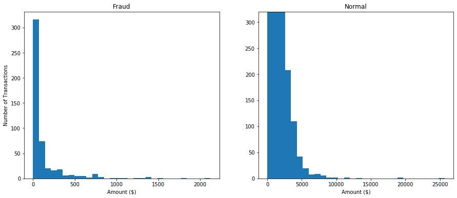
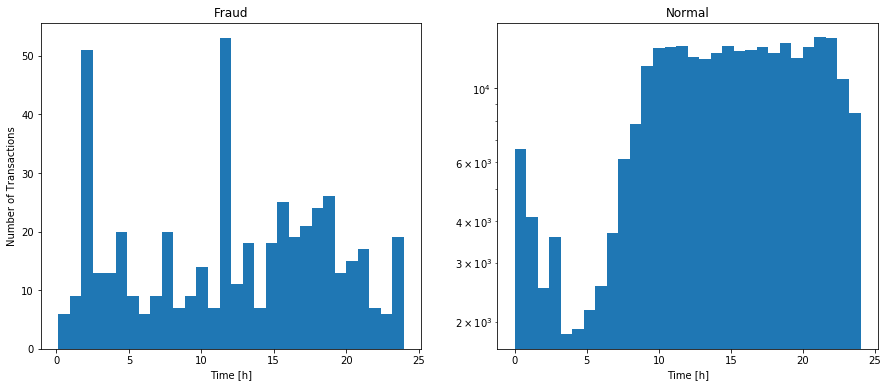
The number of transactions is very different since there are much more normal transactions then frauds. We can just see the differences between the plots. Looking at them, we can see that most frauds happen on small transactions (-500$). However, the “Time” feature can be very informative, on the plots below we can see that most frauds happen at ~2AM and ~12h.
# time comparison - Do fraudulent transactions occur more often during a certain frames?

fig, (ax1, ax2) = plt.subplots(1, 2, figsize=(15, 6))
bins = 30

ax1.hist(df_fraud['Time'], bins=bins)
ax2.hist(df_ok['Time'], bins=bins)

ax1.set_title('Fraud')
ax2.set_title('Normal')

ax1.set_xlabel('Time [h]')
ax2.set_xlabel('Time [h]')
ax1.set_ylabel('Number of Transactions')

ax2.set_yscale('log')
plt.show()
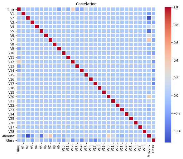
corr = df.corr()

plt.figure(figsize = (10,8))
sns.heatmap(corr, cmap = "coolwarm", linewidth = 2, linecolor = "white")
plt.title("Correlation")
plt.show()
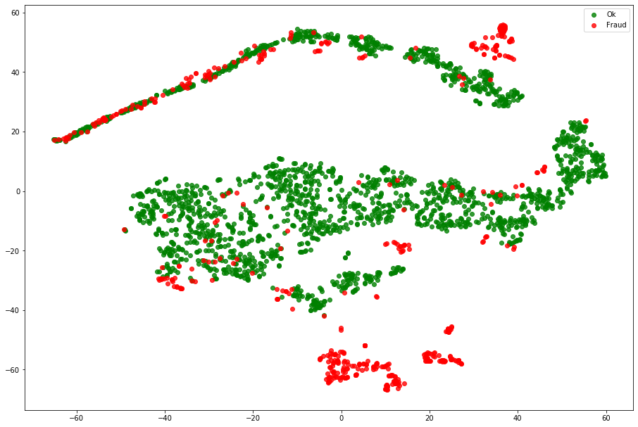
This article proposes an unsupervised approach to detect frauds, the only place the labels are used is to evaluate the algorithm. One of the biggest challenge of this problem is that the target is highly imbalanced as only 0.17% cases are fraudulent transactions. But the advantage of the representation learning approach is that it is still able to handle such imbalance nature of the problems. Using TSNE we can try to see how the transactions are similar:
ok_sample = df[df['Class'] == 0].sample(2000)
df_tsne = ok_sample.append(df_fraud).sample(frac=1).reset_index(drop=True)
X_tsne = df_tsne.drop(['Class'], axis = 1).values
y_tsne = df_tsne["Class"].values

tsne = TSNE(n_components=2, random_state=42, n_jobs=-1)
X_tsne = tsne.fit_transform(X_tsne)
fig = plt.figure(figsize=(12, 8))
ax = fig.add_axes([0, 0, 1, 1])
ax.scatter(X_tsne[np.where(y_tsne == 0), 0], X_tsne[np.where(y_tsne == 0), 1],
           marker='o', color='g', linewidth='1', alpha=0.8, label='Ok')
ax.scatter(X_tsne[np.where(y_tsne == 1), 0], X_tsne[np.where(y_tsne == 1), 1],
           marker='o', color='r', linewidth='1', alpha=0.8, label='Fraud')
ax.legend(loc='best')
<matplotlib.legend.Legend at 0x7f4a73ccc510>
X = df.drop('Class', axis=1)
y = df['Class']
X_train, X_val, y_train, y_val = train_test_split(X, y, stratify=y, test_size=0.2, random_state=42)
X_train.shape, X_val.shape
((227845, 30), (56962, 30))
The main ideia of this approach is to compress the data making a “latent representation” and then reconstruct the data. If a sample is similar to the rest of the dataset, the reconstructed data will be similar or even equal to the original data. However, if the sample is not similar to the rest, the reconstructed sample will not be similar to the original one. In short, we compress the data and reconstruct it. If the reconstructed data is not similar to the original one, we have a fraud.
Using a PCA
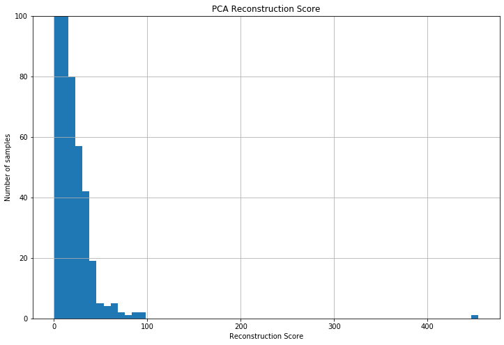
Using Principal component analysis (PCA), we managed to compress the data from 30 features to 10 features and calculated the reconstruction score. The histogram for this score is below:
scores = []
for n in range(2, 31):
    pca = PCA(n_components=n)
    pca.fit(X_train)
    X_tt = pca.transform(X_train)
    X_dt = pca.inverse_transform(X_tt)

    scores.append(mean_squared_error(X_train, X_dt))
scores = np.array(scores)
print(scores.argmin() + 2)
30
n_components = 10
pca = PCA(n_components=n_components)

pca.fit(X_train)
PCA(copy=True, iterated_power='auto', n_components=10, random_state=None,
    svd_solver='auto', tol=0.0, whiten=False)
Train eval
X_tt = pca.transform(X_train)
X_dt = pca.inverse_transform(X_tt)
X_dt = pd.DataFrame(X_dt, columns=X_train.columns, index=X_train.index)

reconstruction_score = []
for idx in X_train.index:
    score = mean_squared_error(X_train.loc[idx], X_dt.loc[idx])
    reconstruction_score.append(score)

rc_scores = pd.DataFrame(reconstruction_score, index=X_train.index, columns=['reconstruction_score'])

rec_mean = rc_scores['reconstruction_score'].mean()
rec_median = rc_scores['reconstruction_score'].median()
rec_std = rc_scores['reconstruction_score'].std()

rc_scores = rc_scores.sort_values(by='reconstruction_score', ascending=False)

top_scores_idx = rc_scores[(rc_scores > (rec_median + 2*rec_std))].dropna().index
train_fraud_index = list(y_train[y_train == 1].index)
plt.figure(figsize=(12, 8))
rc_scores['reconstruction_score'].hist(bins=60)
plt.ylim(0, 100)
plt.title('PCA Reconstruction Score')
plt.xlabel('Reconstruction Score')
plt.ylabel('Number of samples')
Text(0, 0.5, 'Number of samples')
pred = pd.DataFrame(index=X_train.index)
pred['fraud'] = 0
for x in top_scores_idx:
    pred['fraud'].loc[x] = 1

print(classification_report(y_train, pred['fraud']))
print('Rate of transations to investigate:', len(top_scores_idx) / len(X_train) * 100, '%')
              precision    recall  f1-score   support

           0       1.00      1.00      1.00    227451
           1       0.20      0.65      0.31       394

    accuracy                           1.00    227845
   macro avg       0.60      0.82      0.65    227845
weighted avg       1.00      1.00      1.00    227845

Rate of transations to investigate: 0.5508130527332178 %
Val eval
X_tt = pca.transform(X_val)
X_dt = pca.inverse_transform(X_tt)
X_dt = pd.DataFrame(X_dt, columns=X_val.columns, index=X_val.index)

reconstruction_score = []
for idx in X_val.index:
    score = mean_squared_error(X_val.loc[idx], X_dt.loc[idx])
    reconstruction_score.append(score)

rc_scores = pd.DataFrame(reconstruction_score, index=X_val.index, columns=['reconstruction_score'])

rec_mean = rc_scores['reconstruction_score'].mean()
rec_median = rc_scores['reconstruction_score'].median()
rec_std = rc_scores['reconstruction_score'].std()

rc_scores = rc_scores.sort_values(by='reconstruction_score', ascending=False)

top_scores_idx = rc_scores[(rc_scores > (rec_median + 2*rec_std))].dropna().index
val_fraud_index = list(y_val[y_val == 1].index)
pred = pd.DataFrame(index=X_val.index)
pred['fraud'] = 0
for x in top_scores_idx:
    pred['fraud'].loc[x] = 1

print(classification_report(y_val, pred['fraud']))
print('Rate of transations to investigate:', len(top_scores_idx) / len(X_val) * 100, '%')
              precision    recall  f1-score   support

           0       1.00      0.99      1.00     56864
           1       0.17      0.76      0.28        98

    accuracy                           0.99     56962
   macro avg       0.59      0.87      0.64     56962
weighted avg       1.00      0.99      1.00     56962

Rate of transations to investigate: 0.744355886380394 %
Tsne from pca representation
We can see that most samples have a low reconstruction score and then, probably most frauds have more then 50 reconstruction score. Using TSNE we can compare the original data disposition with the PCA compressed data distribution.
X_pca_tsne = pca.transform(X_train)
X_pca_tsne = pd.DataFrame(X_pca_tsne, index=X_train.index)

X_pca_tsne['Class'] = y_train
ok_sample = X_pca_tsne[X_pca_tsne['Class'] == 0].sample(2000)
df_fraud = X_pca_tsne[X_pca_tsne['Class'] == 1]
df_tsne = ok_sample.append(df_fraud).sample(frac=1).reset_index(drop=True)

X_tsne = df_tsne.values
y_tsne = df_tsne["Class"].values

tsne = TSNE(n_components=2, random_state=42, n_jobs=-1)
X_tsne = tsne.fit_transform(X_tsne)
fig = plt.figure(figsize=(12, 8))
ax = fig.add_axes([0, 0, 1, 1])
ax.scatter(X_tsne[np.where(y_tsne == 0), 0], X_tsne[np.where(y_tsne == 0), 1],
           marker='o', color='g', linewidth='1', alpha=0.8, label='Ok')
ax.scatter(X_tsne[np.where(y_tsne == 1), 0], X_tsne[np.where(y_tsne == 1), 1],
           marker='o', color='r', linewidth='1', alpha=0.8, label='Fraud')
ax.legend(loc='best')
<matplotlib.legend.Legend at 0x7f4a6d7a9650>
Now, we need to set a threshold to the reconstruction score. Usualy there domain expertise is used to help to set this threshold since it impacts direcly on the precision and recall trade-off. Using the mean and standard deviation of the reconstruction score we can set a reasonable threshold. Then, I choose to set the threshold to mean + 2*std. With this, auditing 0.74% of the transactions we managed to find 87% of the frauds.
Using a Autoencoder
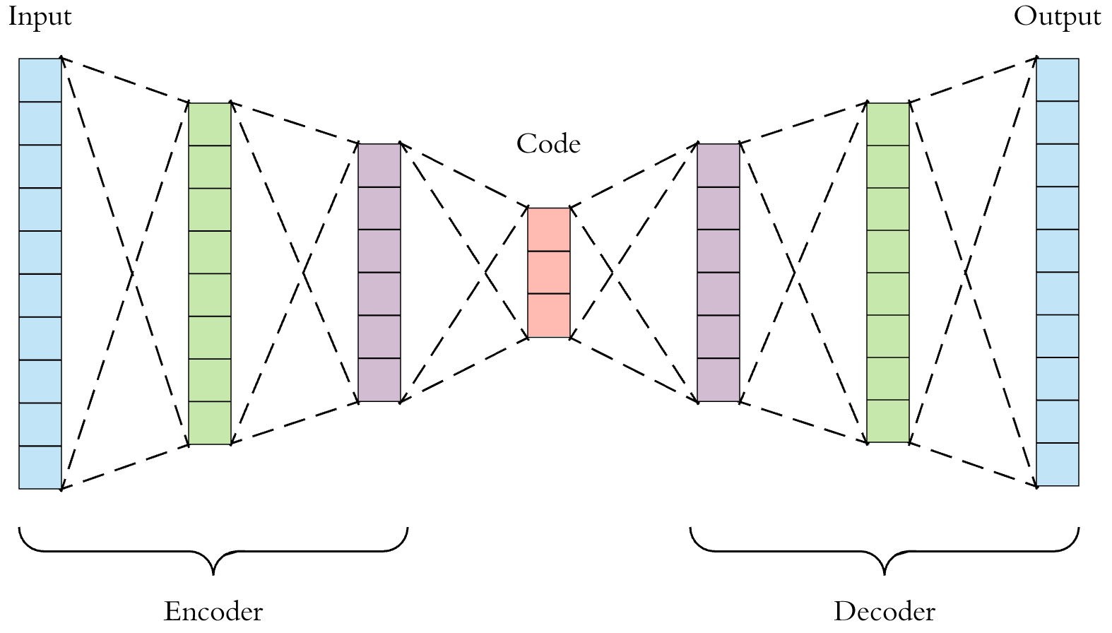
An autoencoder is a type of artificial neural network used to learn efficient data codings in an unsupervised manner. It is composed of a enconding part responsable to compress the data and a decoder to reconstruct the data.
ss = StandardScaler()
X_tscaled = ss.fit_transform(X_train.values)
X_train = pd.DataFrame(X_tscaled, columns=X_train.columns, index=X_train.index)

X_vscaled = ss.transform(X_val.values)
X_val = pd.DataFrame(X_vscaled, columns=X_val.columns, index=X_val.index)
# input
inp = Input(shape=(X.shape[1],))

# Encoder
x = Dense(100, activation='relu')(inp)
x = Dense(50, activation='relu')(x)

# Decoder
x = Dense(50, activation='tanh')(x)
x = Dense(100, activation='tanh')(x)

## output
output = Dense(X.shape[1], activation='relu')(x)

autoencoder = Model(inp, output)

lr = 0.0001
epochs = 300
adam = Adam(lr=lr, decay=(lr/epochs))

autoencoder.compile(optimizer=adam, loss="mean_squared_error")
autoencoder.summary()
Model: "model"
_________________________________________________________________
Layer (type)                 Output Shape              Param #
=================================================================
input_1 (InputLayer)         [(None, 30)]              0
_________________________________________________________________
dense (Dense)                (None, 100)               3100
_________________________________________________________________
dense_1 (Dense)              (None, 50)                5050
_________________________________________________________________
dense_2 (Dense)              (None, 50)                2550
_________________________________________________________________
dense_3 (Dense)              (None, 100)               5100
_________________________________________________________________
dense_4 (Dense)              (None, 30)                3030
=================================================================
Total params: 18,830
Trainable params: 18,830
Non-trainable params: 0
_________________________________________________________________
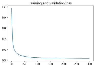
history = autoencoder.fit(X_train.values, X_train.values, batch_size=2048, epochs=epochs,
                          shuffle=True, verbose=0)
loss = history.history['loss']

ts = range(epochs)

plt.plot(ts, loss)
plt.title('Training and validation loss')
Text(0.5, 1.0, 'Training and validation loss')
encoder = Sequential()
encoder.add(autoencoder.layers[0])
encoder.add(autoencoder.layers[1])
encoder.add(autoencoder.layers[2])

decoder = Sequential()
decoder.add(autoencoder.layers[3])
decoder.add(autoencoder.layers[4])
decoder.add(autoencoder.layers[5])
Train eval
X_tt = encoder.predict(X_train)
X_dt = decoder.predict(X_tt)
X_dt = pd.DataFrame(X_dt, columns=X_train.columns, index=X_train.index)

reconstruction_score = []
for idx in X_train.index:
    score = mean_squared_error(X_train.loc[idx], X_dt.loc[idx])
    reconstruction_score.append(score)

rc_scores = pd.DataFrame(reconstruction_score, index=X_train.index, columns=['reconstruction_score'])

rec_mean = rc_scores['reconstruction_score'].mean()
rec_median = rc_scores['reconstruction_score'].median()
rec_std = rc_scores['reconstruction_score'].std()
rc_scores = rc_scores.sort_values(by='reconstruction_score', ascending=False)

top_scores_idx = rc_scores[(rc_scores > (rec_median + 2*rec_std))].dropna().index
train_fraud_index = list(y_train[y_train == 1].index)
pred = pd.DataFrame(index=X_train.index)
pred['fraud'] = 0
for x in top_scores_idx:
    pred['fraud'].loc[x] = 1

print(classification_report(y_train, pred['fraud']))
print('Rate of transations to investigate:', len(top_scores_idx) / len(X_train) * 100, '%')
              precision    recall  f1-score   support

           0       1.00      1.00      1.00    227451
           1       0.17      0.57      0.27       394

    accuracy                           0.99    227845
   macro avg       0.59      0.78      0.63    227845
weighted avg       1.00      0.99      1.00    227845

Rate of transations to investigate: 0.571880006144528 %
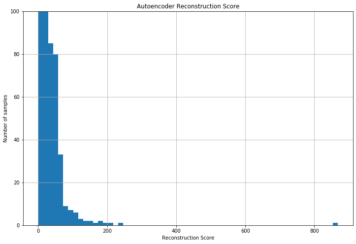
The aim of an autoencoder is to learn a representation (encoding) for a set of data, typically for the purpose of dimensionality reduction. Analogously to the PCA approach, the reconstrcution score histogram can be seen below:
plt.figure(figsize=(12, 8))
rc_scores['reconstruction_score'].hist(bins=60)
plt.ylim(0, 100)
plt.title('Autoencoder Reconstruction Score')
plt.xlabel('Reconstruction Score')
plt.ylabel('Number of samples')
Text(0, 0.5, 'Number of samples')
val eval
X_tt = encoder.predict(X_val)
X_dt = decoder.predict(X_tt)
X_dt = pd.DataFrame(X_dt, columns=X_val.columns, index=X_val.index)

reconstruction_score = []
for idx in X_val.index:
    score = mean_squared_error(X_val.loc[idx], X_dt.loc[idx])
    reconstruction_score.append(score)

rc_scores = pd.DataFrame(reconstruction_score, index=X_val.index, columns=['reconstruction_score'])

rec_mean = rc_scores['reconstruction_score'].mean()
rec_median = rc_scores['reconstruction_score'].median()
rec_std = rc_scores['reconstruction_score'].std()
rc_scores = rc_scores.sort_values(by='reconstruction_score', ascending=False)

top_scores_idx = rc_scores[(rc_scores > (rec_median + 2*rec_std))].dropna().index
train_fraud_index = list(y_train[y_train == 1].index)
pred = pd.DataFrame(index=X_val.index)
pred['fraud'] = 0
for x in top_scores_idx:
    pred['fraud'].loc[x] = 1

print(classification_report(y_val, pred['fraud']))
print('Rate of transations to investigate:', len(top_scores_idx) / len(X_val) * 100, '%')
              precision    recall  f1-score   support

           0       1.00      0.99      1.00     56864
           1       0.13      0.65      0.22        98

    accuracy                           0.99     56962
   macro avg       0.57      0.82      0.61     56962
weighted avg       1.00      0.99      0.99     56962

Rate of transations to investigate: 0.8514448228643657 %
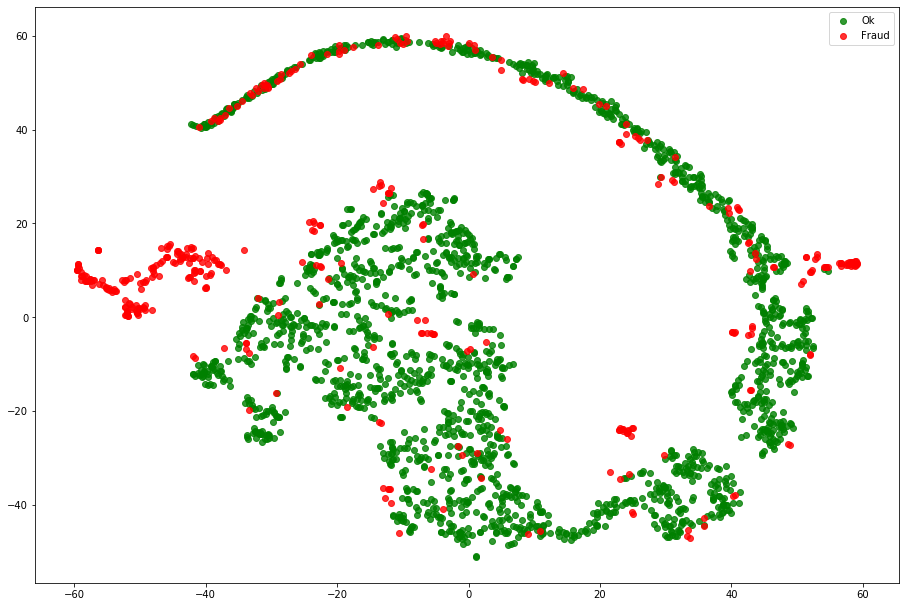
Tsne
We can see that most samples have a low reconstruction score and then, probably most frauds have more then ~60 reconstruction score. Using TSNE we can compare the original data disposition with the Autoencoder compressed data distribution.
X_enc_tsne = encoder.predict(X_train)
X_enc_tsne = pd.DataFrame(X_enc_tsne, index=X_train.index)

X_enc_tsne['Class'] = y_train
ok_sample = X_enc_tsne[X_enc_tsne['Class'] == 0].sample(2000)
df_fraud = X_enc_tsne[X_enc_tsne['Class'] == 1]
df_tsne = ok_sample.append(df_fraud).sample(frac=1).reset_index(drop=True)

X_tsne = df_tsne.values
y_tsne = df_tsne["Class"].values

tsne = TSNE(n_components=2, random_state=42, n_jobs=-1)
X_tsne = tsne.fit_transform(X_tsne)
fig = plt.figure(figsize=(12, 8))
ax = fig.add_axes([0, 0, 1, 1])
ax.scatter(X_tsne[np.where(y_tsne == 0), 0], X_tsne[np.where(y_tsne == 0), 1],
           marker='o', color='g', linewidth='1', alpha=0.8, label='Ok')
ax.scatter(X_tsne[np.where(y_tsne == 1), 0], X_tsne[np.where(y_tsne == 1), 1],
           marker='o', color='r', linewidth='1', alpha=0.8, label='Fraud')
ax.legend(loc='best')
<matplotlib.legend.Legend at 0x7f4a73125350>
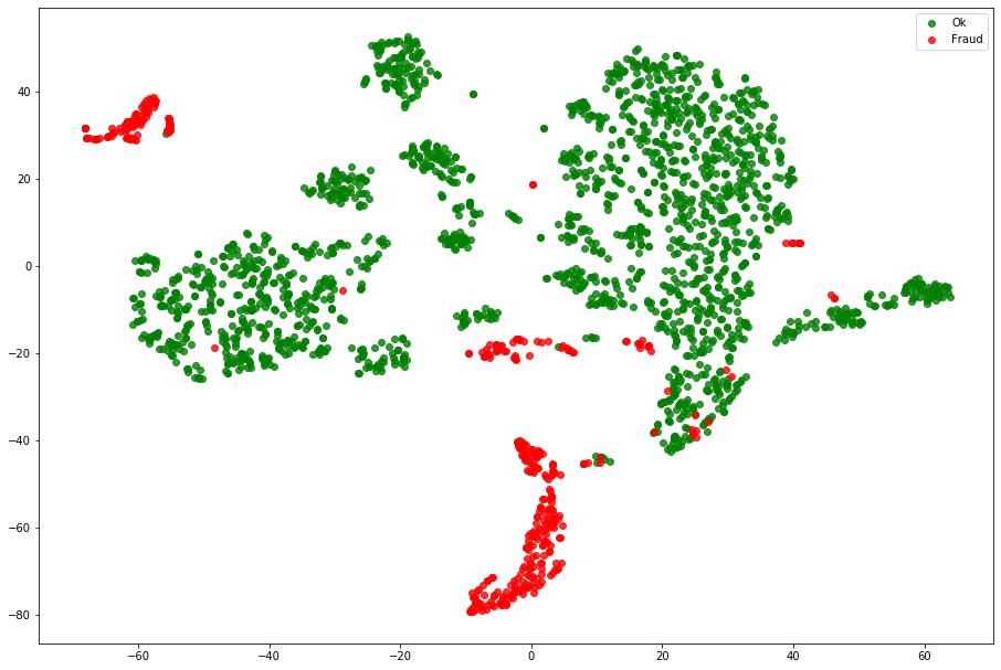
The Autoencoder representation seens to split quite well the frauds from the normal data. Now, we need to set a threshold to the reconstruction score. Usualy there domain expertise is used to help to set this threshold since it impacts direcly on the precision and recall trade-off. Using the mean and standard deviation of the reconstruction score we can set a reasonable threshold. Then, I choose to set the threshold to mean + 2*std. With this, auditing 0.85% of the transactions we managed to find 65% of the frauds.
Conclusion
The objective of the approach was fulfilled, making possible to detect frauds with an 100% unsupervised approach. Nevertheless, there are several ways to make this approach work better, like:
- Tunning the used models (PCA and Autoencoder);
- Tune the threshold of reconstruction score;
- Explore if the PCA and Autoencoder are detecting the same frauds. If they work in different ways, maybe it is -worth to make an emsamble;
- Augment the data with some feature engineering.